LLM结构的学习路径

• LLM结构解析(开源LlaMA)
• 自定义数据集构造
• 自定义损失函数和模型训练/微调

Transformer经典结构

• Encoder-decoder结构
• 输入部分
  • Input embedding
  • Positional embedding
• Transformer部分
  • Attention
  • Feed forward

LlaMA的模型结构

HF LlaMA模型结构

LlamaForCausalLM(
  (model): LlamaModel(
    (embed_tokens): Embedding(128256, 2048)
    (layers): ModuleList(
      (0-15): 16 x LlamaDecoderLayer(
        (self_attn): LlamaAttention
        (mlp): LlamaMLP
        (input_layernorm): LlamaRMSNorm
        (post_attention_layernorm): LlamaRMSNorm
    )
    (norm): LlamaRMSNorm((2048,), eps=1e-05)
    (rotary_emb): LlamaRotaryEmbedding()
  )
  (lm_head): Linear(in_features=2048, out_features=128256, bias=False)
)

LlamaDecoderLayer内部结构

(self_attn): LlamaAttention(
  (q_proj): Linear(in_features=2048, out_features=2048, bias=False)
  (k_proj): Linear(in_features=2048, out_features=512, bias=False)
  (v_proj): Linear(in_features=2048, out_features=512, bias=False)
  (o_proj): Linear(in_features=2048, out_features=2048, bias=False)
  (rotary_emb): LlamaRotaryEmbedding()
)
(mlp): LlamaMLP(
  (gate_proj): Linear(in_features=2048, out_features=8192, bias=False)
  (up_proj): Linear(in_features=2048, out_features=8192, bias=False)
  (down_proj): Linear(in_features=8192, out_features=2048, bias=False)
  (act_fn): SiLU()
)
(input_layernorm): LlamaRMSNorm((2048,), eps=1e-05)
(post_attention_layernorm): LlamaRMSNorm((2048,), eps=1e-05)

Qwen3-0.6B模型结构

Qwen3ForCausalLM(
  (model): Qwen3Model(
    (embed_tokens): Embedding(151936, 1024)
    (layers): ModuleList(
      (0-27): 28 x Qwen3DecoderLayer(
        (self_attn): Qwen3Attention()
        (mlp): Qwen3MLP()
        (input_layernorm): Qwen3RMSNorm((1024,), eps=1e-06)
        (post_attention_layernorm): Qwen3RMSNorm((1024,), eps=1e-06)
      )
    )
    (norm): Qwen3RMSNorm((1024,), eps=1e-06)
    (rotary_emb): Qwen3RotaryEmbedding()
  )
  (lm_head): Linear(in_features=1024, out_features=151936, bias=False)
)

Qwen3Attention内部结构

(q_proj): Linear(in_features=1024, out_features=2048, bias=False)
(k_proj): Linear(in_features=1024, out_features=1024, bias=False)
(v_proj): Linear(in_features=1024, out_features=1024, bias=False)
(o_proj): Linear(in_features=2048, out_features=1024, bias=False)
(q_norm): Qwen3RMSNorm((128,), eps=1e-06)
(k_norm): Qwen3RMSNorm((128,), eps=1e-06)

Qwen3MLP内部结构

(gate_proj): Linear(in_features=1024, out_features=3072, bias=False)
(up_proj): Linear(in_features=1024, out_features=3072, bias=False)
(down_proj): Linear(in_features=3072, out_features=1024, bias=False)
(act_fn): SiLU()

架构新进展：DeepSeek-V4.1-Flash

来源：DeepSeek-V4.1-Flash 技术报告，Figure 3，§2（架构）

DeepSeek-V4.1-Flash：架构要点

• CED：降低长输入的处理成本
  20 层因果 Encoder + 20 层 Decoder；后者的全局 KV 来自 Encoder 输出，大部分输入可跳过后半网络的完整计算。
• CSA2：跨层复用历史信息
  Full 建立全局 KV，Reindex 共享 KV 并重新检索，Reuse 同时复用 KV 和所选位置；各层仍保留自己的 Q 与局部滑窗。
• 面向长上下文的组合优化
  分层索引缩小检索范围，FP4 压缩全局主 KV；重放末尾 128 个 token，近似恢复局部滑窗状态。

回到本讲：文本仍先查表得到 embedding；位置关系仍需在 attention 中编码。

本次课程关注

• 目前，流行结构多为Decoder-only
• 输入部分
  • Input embedding
  • Positional embedding
• Transformer部分
  • Attention
  • Feed forward

为LLM构建词汇表

• 自然语言是离散的，LLM词汇表依然延续离散的模式构建
• 如何分词: 'Hello, world!'
  • word-based: | hello | , | world | ! |
  • character-based: h|e|l|l|o|,|w|o|r|l|d|!
  • subword-based tokenization
    • 基本原则：常用“词”不拆分，一般词分解为有意义的子词(subword)
    • 来试试Tiktokenizer

中文、英文与混合文本

语言差异发生在 tokenizer 阶段；后面的 embedding 只处理统一的 token ID。token 数量会影响上下文长度、显存和推理成本。

观察中英文分词

使用同一个 Qwen3 tokenizer，比较中英文和混合文本：

for text in ["Nanjing University", "南京大学", "LLM中的embedding"]:
    ids = tokenizer.encode(text, add_special_tokens=False)
    print(text, tokenizer.tokenize(text), ids, len(ids))
    assert tokenizer.decode(ids) == text

• token 字符串可能是字节的内部表示，不一定直接可读。

批量输入：补齐与 attention mask

if tokenizer.pad_token_id is None:
    tokenizer.pad_token = tokenizer.eos_token
batch = tokenizer(["你好", "南京大学"], padding=True,
                  return_tensors="pt")
print("token IDs:\n", batch["input_ids"])
print("mask:\n", batch["attention_mask"])

批量输入：补齐与 attention mask

Qwen3 实际输出（右侧补齐）：

                  input_ids          attention_mask
你好              [108386, 151643]    [1, 0]
南京大学          [102034,  99562]    [1, 1]

两者形状均为 [b, s]。1 是有效位置，0 是补齐位置。
这里 151643 是补齐 token；0/1 mask 不能直接加到 attention 分数上。

Input embedding

(embed_tokens): Embedding(128256, 2048)

• tokenizer：将自然语言转换为 token ID
• embedding：根据 token ID 查表，得到稠密向量表示
• 每个index对应一个embedding
  • embedding需训练
• 例如：
  • 用户给LLM的输入: "你好，请介绍下南京大学"
  • LLM经过预训练的embedding: [[0.2234234,-0.28178,...], [...]]

Input embedding原理

"语言是文明的载体，对人类而言是这样，对LLM而言也是这样"

Input embedding原理

这也是"南京大学"

Input embedding原理

这也是“南京大学”：南大的(部分)特征

Input embedding原理

Input embedding：构建表达自然语言特征的表示 (representation)

位置编码 (Positional embeddings)

位置编码：用来标记每个词的位置

• Sinusoidal PE
  • Attention is all you need时代的位置编码
• Rotary PE(旋转位置编码)
  • 基于论文RoFormer

位置编码的初衷

• Attention模块计算的是每个token的注意力分数
  • 衡量token与token之间的相关性
• 位置编码用来标记每个token的位置
  • 让LLM更好的建模不同位置的token之间的关系

绝对位置编码

直接在每个token的embedding上线性叠加位置编码: ，其中为可训练的向量

位置编码与序数编码的关联

• 序数表示次序，位置编码的用意也在于此。例如从小就学的序数编码：
  • 十进制: 1 2 3 4 5 6 7 8 9 10, ...
  • 二进制: 0, 1, 10, 11, 100, 101, 110, 111, 1000, 1001, ...
• 但是：
  • LLM中的token embedding为向量,如何构造型为向量的位置编码？

序数的周期性

十进制本身是周期性的，二进制也是周期性的

Sinusodial PE

构建n维的位置编码，每一维用不同的周期函数刻画取值

旋转位置编码（Rotary PE）

Rotary PE 的 2D 理解：把向量看成箭头

先只看二维向量 。把它画成平面上的一支箭头，位置 不再通过加一个新向量表示，而是让箭头旋转：

x = (1, 0), θ = 30°
位置 0：旋转 0°   → (1, 0)
位置 1：旋转 30°  → (cos 30°, sin 30°)
位置 2：旋转 60°  → (cos 60°, sin 60°)

RoPE：位置改变方向，长度保持不变

旋转不会改变向量长度：

因此，同一个 token 在不同位置有不同方向，但不会因为位置编码而改变向量的尺度。

• 位置 0：
• 位置 1：
• 位置 2：

RoPE 为什么能表达相对位置？

设 位于位置 ， 位于位置 。attention 中的点积满足：

结果只依赖位置差 ，所以 attention 可以感知两个 token 相距多远。

RoPE 给每个位置配一个旋转角度；Q 和 K 比较旋转后的方向时，结果自然包含相对距离信息。

从二维推广到高维

高维 RoPE 将 hidden vector 的维度两两分组：、、……，每一对维度在自己的二维平面中旋转。

不同维度使用不同的角速度，因此同时表达短距离和长距离的位置变化。实际模型在 attention 的每一层对 Q 和 K 应用 RoPE。

RoPE实现

RoPE的2D实现

RoPE的n维实现

Rotary PE的可视化展示

RoPE在LlaMA中的构建

不同于经典Transformers结构，只对输入的token做位置编码的叠加

LlaMA中的RoPE在Transformer的每一层都会对Q和K进行位置编码的叠加

补充内容：PyTorch Tensor操作详解

在深度学习中，tensor操作是构建模型的基础。理解各种tensor操作对于实现LLM等复杂模型至关重要。

Tensor操作分类

• 形状变换操作
  • view() / reshape() - 改变tensor形状
  • transpose() / permute() - 转置和维度重排
  • squeeze() / unsqueeze() - 压缩/扩展维度
• 数学运算操作
  • matmul() / @ - 矩阵乘法
  • bmm() - 批量矩阵乘法
  • einsum() - 爱因斯坦求和约定
• 存储连续：contiguous()

Tensor操作分类

• 索引和切片操作
  • gather() / scatter() - 按索引收集/分散
  • index_select() - 按索引选择
  • masked_select() - 按掩码选择

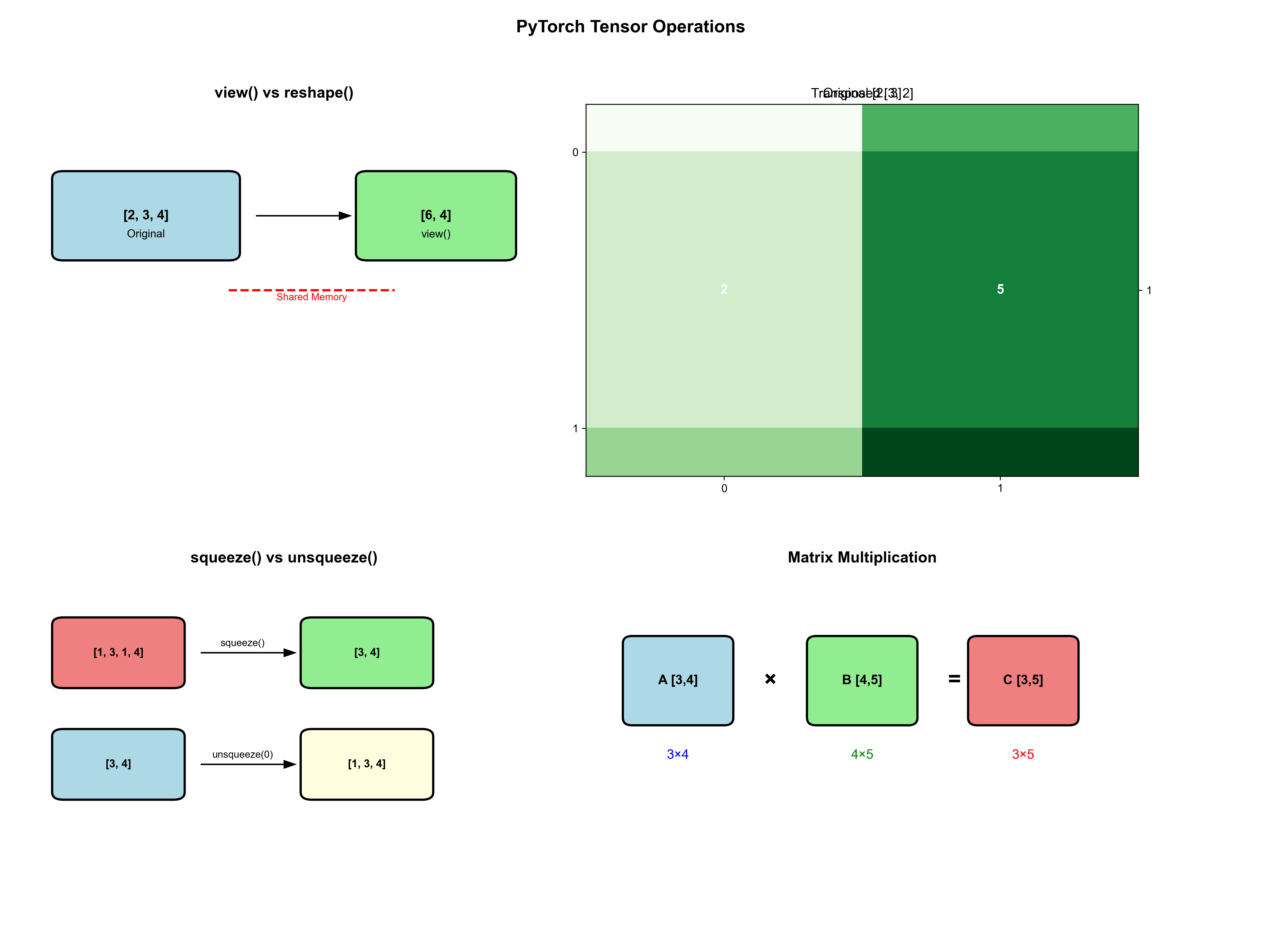
形状变换操作：view vs reshape

基本原理

• view(): 返回与原tensor共享存储的新视图，要求tensor在内存中连续
• reshape(): 如果可能则返回view，否则返回副本

代码示例

# view() - 要求tensor连续
x = torch.randn(2, 3, 4)
y = x.view(6, 4)  # 成功：2*3=6

# 如果tensor不连续，view()会报错
x_transposed = x.transpose(0, 1)  # 不连续
# y = x_transposed.view(12, 2)  # 报错！

# reshape() - 自动处理连续性问题
y = x_transposed.reshape(12, 2)  # 成功：自动处理

转置操作：transpose vs permute

transpose() - 交换两个维度

x = torch.randn(2, 3, 4, 5)
y = x.transpose(1, 3)  # 交换维度1和3
print(x.shape)  # torch.Size([2, 3, 4, 5])
print(y.shape)  # torch.Size([2, 5, 4, 3])

permute() - 重新排列所有维度

x = torch.randn(2, 3, 4, 5)
y = x.permute(0, 3, 1, 2)  # 重新排列维度
print(x.shape)  # torch.Size([2, 3, 4, 5])
print(y.shape)  # torch.Size([2, 5, 3, 4])

维度操作：squeeze vs unsqueeze

squeeze() - 移除大小为1的维度

x = torch.randn(1, 3, 1, 4)
y = x.squeeze()  # 移除所有大小为1的维度
z = x.squeeze(0)  # 只移除第0维
print(x.shape)  # torch.Size([1, 3, 1, 4])
print(y.shape)  # torch.Size([3, 4])
print(z.shape)  # torch.Size([3, 1, 4])

维度操作：squeeze vs unsqueeze

unsqueeze() - 在指定位置插入大小为1的维度

x = torch.randn(3, 4)
y = x.unsqueeze(0)  # 在第0维插入
z = x.unsqueeze(-1)  # 在最后一维插入
print(x.shape)  # torch.Size([3, 4])
print(y.shape)  # torch.Size([1, 3, 4])
print(z.shape)  # torch.Size([3, 4, 1])

Broadcasting（广播）机制

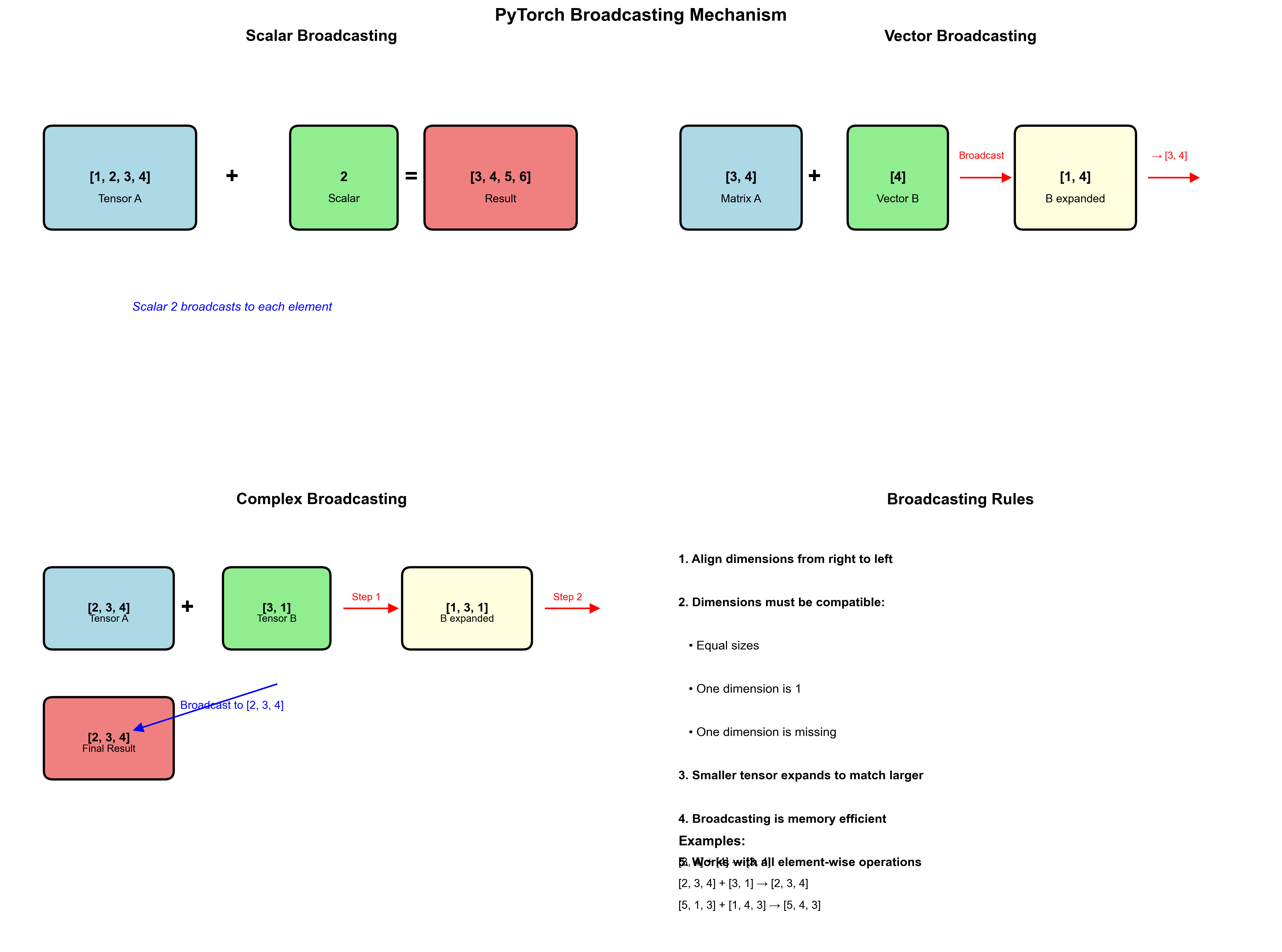
Broadcasting是PyTorch中一种强大的机制，允许不同形状的tensor进行运算。它遵循以下规则：

1. 从右向左对齐维度：从最后一个维度开始比较
2. 维度兼容性：两个维度要么相等，要么其中一个为1，要么其中一个不存在
3. 自动扩展：较小的tensor会在不兼容的维度上自动扩展

Broadcasting规则示例

# 示例1: 标量与tensor
a = torch.tensor([1, 2, 3])
b = 2
c = a + b  # [3, 4, 5] - 标量自动广播到每个元素

# 示例2: 不同形状的tensor
A = torch.randn(3, 4)      # [3, 4]
B = torch.randn(4)         # [4]
C = A + B                  # [3, 4] - B自动扩展为[1, 4]然后[3, 4]

# 示例3: 更复杂的广播
A = torch.randn(2, 3, 4)   # [2, 3, 4]
B = torch.randn(3, 1)      # [3, 1]
C = A + B                  # [2, 3, 4] - B扩展为[1, 3, 1]然后[2, 3, 4]

Broadcasting在深度学习中的应用

# 1. 添加偏置项
x = torch.randn(32, 128)  # [batch_size, features]
bias = torch.randn(128)   # [features]
y = x + bias              # 每个样本都加上相同的偏置

# 2. 注意力机制中的mask
scores = torch.randn(2, 8, 8)  # [batch, seq_len, seq_len]
mask = torch.tensor([1, 1, 1, 0, 0, 0, 0, 0])  # [seq_len]
masked_scores = scores.masked_fill(~mask.bool().view(1, 1, -1), float("-inf"))  # 广播到[2, 8, 8]

# 3. 批量归一化
x = torch.randn(32, 64, 28, 28)  # [batch, channels, height, width]
mean = torch.mean(x, dim=(0, 2, 3), keepdim=True)  # [1, 64, 1, 1]
normalized = (x - mean) / torch.std(x, dim=(0, 2, 3), keepdim=True)

矩阵乘法操作

不同矩阵乘法的使用场景

• torch.matmul() / @: 通用矩阵乘法，支持广播
• torch.bmm(): 批量矩阵乘法，专门用于3D tensor
• torch.mm(): 2D矩阵乘法

# 批量矩阵乘法
A_batch = torch.randn(2, 3, 4)
B_batch = torch.randn(2, 4, 5)
C_batch = torch.bmm(A_batch, B_batch)
print(C_batch.shape)  # torch.Size([2, 3, 5])

爱因斯坦求和约定 (einsum)

einsum提供了一种简洁的方式来表达复杂的tensor操作：

# 矩阵乘法: C[i,j] = sum_k A[i,k] * B[k,j]
A = torch.randn(3, 4)
B = torch.randn(4, 5)
C = torch.einsum('ik,kj->ij', A, B)
# 批量矩阵乘法
A_batch = torch.randn(2, 3, 4)
B_batch = torch.randn(2, 4, 5)
C_batch = torch.einsum('bik,bkj->bij', A_batch, B_batch)
# 注意力机制中的QK^T计算
Q = torch.randn(2, 8, 64)  # [batch, seq_len, d_model]
K = torch.randn(2, 8, 64)
scores = torch.einsum('bqd,bkd->bqk', Q, K)

索引和选择操作

gather() - 按索引收集元素

# 在指定维度上按索引收集元素
x = torch.randn(3, 4)
indices = torch.tensor([0, 2, 1])
y = torch.gather(x, 1, indices.unsqueeze(1))
print(x)
print(y)  # 每行按indices选择元素

scatter() - 按索引分散元素

# 将元素分散到指定位置
x = torch.zeros(3, 4)
values = torch.randn(3, 2)
indices = torch.tensor([[0, 2], [1, 3], [0, 1]])
x.scatter_(1, indices, values)
print(x)

拓展阅读&参考文档

Hugging Face
Accelerating a Hugging Face Llama 2 and Llama 3 models with Transformer Engine

RoPE部分
Transformer升级之路：10、RoPE是一种β进制编码. 苏剑林
RoFormer: Enhanced Transformer with Rotary Position Embedding

PyTorch Tensor操作
PyTorch官方文档 - Tensor操作
Einops库 - 更优雅的tensor操作